Table of Contents
We have include a descriptions of the different demos than can be found in the library. Most of them are used to highlight the capabilities of the Bayesian optimization framework or the characteristics of the library.
Important: Some demos requires extra dependencies to work. They will be mention in each demo.
C/C++ demos
These demos are automatically compiled and installed with the library. They can be found in the /bin subfolder. The source code of these demos is in /examples
Quadratic examples (continuous and discrete)
bo_cont and bo_disc provides examples of the C (callback) and C++ (inheritance) interfaces for a simple quadratic function. They are the best starting point to start playing with the library.
Interactive 1D test
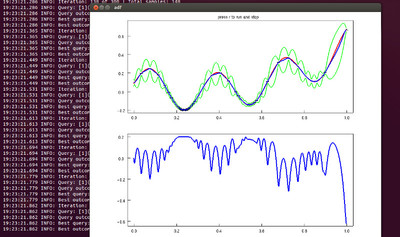
bo_oned deals with a more interesting, yet simple, multimodal 1D function. bo_display shows the same example, but includes an interactive visualization tool to show the features of different configurations, like different surrogate and criteria functions (Important: bo_display requires CMake to find OpenGL and GLUT/FreeGLUT to be compiled).
Note: For some NVIDIA setups, you might need to preload the Pthreads dynamic library. For example, in Linux
>> LD_PRELOAD=/lib/x86_64-linux-gnu/libpthread.so.0 ./bin/bo_display
Standalone optimization module
BayesOpt can also be used to optimize a standalone application either using CLI for sending parameters and receiving output (see branin_system_call) or by using XML files to message passing (see branin_xml). Both demos use the Branin function defined in the next section.
Standard nonlinear function benchmarks
Branin function
bo_branin_* are different examples using the 2D Branin function, which is a standard function to evaluate nonlinear optimization algorithms.
![\[ f(x,y) = \left(y-\frac{5.1}{4\pi^2}x^2 + \frac{5}{\pi}x-6\right)^2 + 10\left(1-\frac{1}{8\pi}\right) \cos(x) + 10 \]](form_0.png)
with a search domain  ,
,  .
.
For simplicity to display and use the function, the function used in the code has already been normalized in the [0,1] interval. Then, the function has three global minimum. The position of those points (after normalization) are:

bo_branin use sporadically an empirical estimator (MAP) for kernel hyperparameters. Really fast.
bo_branin_mcmc use continuously a Bayesian estimator (MCMC) for kernel hyperparameters. Much slower but much more robuts. Although for this function the robustness is not as critical, it might be an issue for more complex or high-dimensional functions.
Hartmann6 function
bo_hartmann_* are different examples using the 6D Hartmann function, which is a standard function to evaluate nonlinear optimization algorithms.

with a search domain  .
.
The global minimum is:
![\[ \mathbf{x}^* = \left(0.2069, 0.150011, 0.476874, 0.275332, 0.311652, 0.6573 \right) \qquad \qquad f(\mathbf{x}^*) = -3.32237 \]](form_6.png)
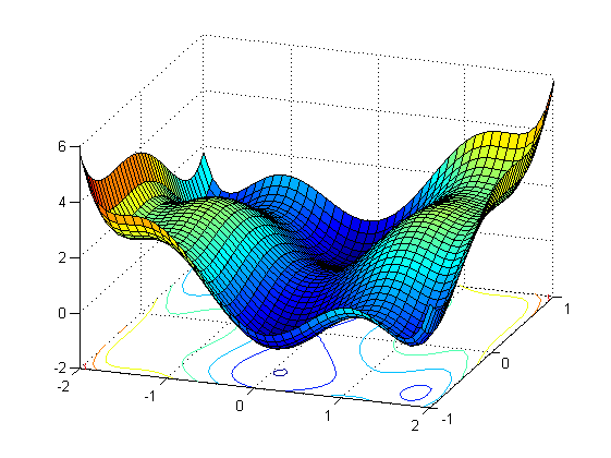
Camelback function
bo_camel_* are different examples using the 2D Camelback function, which is a standard function to evaluate nonlinear optimization algorithms.
![\[ f(x,y) = \left(4 - 2.1x^2 + \frac{x^4}{3}\right) x^2 + x y + \left(-4 + 4y^2\right) y^2 \]](form_7.png)
with a search domain  ,
,  .
.
There are two global minima:

Python demos
These demos use the Python interface of the library. They can be found in the /python subfolder.
Make sure that the interface has been generated and that it can be found in the corresponding path (i.e. PYTHONPATH).
Interface test
demo_quad provides an simple example (quadratic function). It shows the continuous and discrete cases and it also compares the standard (Cython) and the object oriented interfaces. It is the best starting point to start playing with the Python interface.
demo_dimscaling shows a 20 dimensional quadratic function with different smoothness in each dimension. It also show the speed of the library for high dimensional functions.
demo_distance is equivalent to the demo_quad example, but it includes a penalty term with respect to the distance between the current and previous sample. For example, it can be used to model sampling strategies which includes a mobile agent, like a robotic sensor as seen in [Marchant2012].
Multiprocess demo
demo_multiprocess is a simple example that combines BayesOpt with the standard Python multiprocessing library. It shows how simple BayesOpt can be used in a parallelized setup, where one process is dedicated for the BayesOpt and the rests are dedicated to function evaluations. Also, it shows that BayesOpt is thread-safe.
Computer Vision demo
demo_cam is a demonstration of the potetial of BayesOpt for parameter tuning. The advantage of using BayesOpt versus traditional strategies is that it only requires knowledge of the desired behavior, while traditional methods for parameter tuning requires deep knowledge of the algorithm and the meaning of the parameters.
In this case, it takes a simple example (image binarization) and show how optimizing a simple behavior (balanced white/black result) could match the result of the adaptive thresholding from Otsu's method -default in SimpleCV-. Besides, it finds the optimal with few samples (typically between 10 and 20). It can also be used as reference for hyperparameter optimization.
demo_cam requires SimpleCV and a compatible webcam.
MATLAB/Octave demos
These demos use the Matlab interface of the library. They can be found in the /matlab subfolder.
Make sure that the interface has been generated. If the library has been generated as a shared library, make sure that it can be found in the corresponding path (i.e. LD_LIBRARY_PATH in Linux/MacOS) before running MATLAB/Octave.
Interface test
demo_test shows the discrete and continuous interface. The objective function can be selected among all the functions defined in the /matlab/testfunctions subfolder, which includes a selection of standard test functions for nonlinear optimization. By default, the test run these functions:
- Branin
- Quadratic function (discrete version)
- Hartmann 6D
However, these functions are also available for testing:
- Ackley
- Camelback
- Langermann
- Michaelewicz
- Rosenbrock
Demo in very high dimensions
demo_rembo evaluates the REMBO (Random EMbedding Bayesian Optimization) algorithm for optimization in very high dimensions. The idea is that Bayesian optimization can be used very high dimensions provided that the effective dimension is embedded in a lower space, by using random projections.
In this case, we test it against an artificially augmented Branin function with 1000 dimensions where only 2 dimensions are actually relevant (but unknown). The function is defined in the file: braninghighdim
For details about REMBO, see [ZiyuWang2013].